Mass, Momentum, Force and Motion
- Elementary Physics 4
Mass
Mass is a scalar measure of the amount of matter in an object. It is a fundamental property of matter and is invariant under any change of frame of reference. Mass of an object is often denoted by the symbol $m$. SI unit of mass is the kilogram ($\mathrm{kg}$).
Momentum
Momentum is a vector quantity defined as the product of an object’s mass and its velocity. The momentum $\b{p}$ of an object with mass $m$ and velocity $\b{v}$ is given by:
\[ \bs{p} = m \bs{v} \]
SI unit of momentum is kilogram metre per second ($\mathrm{kg \cdot m/s}$).
Force
Force is a vector quantity that represents the interaction between objects, causing them to accelerate. A force $\b{F}$ acting on an object with momentum $\b{p}$ is defined as the rate of change of momentum with respect to time:
\[ \b{F} = \odv{\b{p}}{t} \]
SI unit of force is the newton ($\mathrm{N}$), which is defined as $\mathrm{N} = \mathrm{kg \cdot m/s^2}$.
Free Body Diagram
A free body diagram is a graphical representation used to visualize the forces acting on an object. It shows the object as a point and the forces acting on it as arrows pointing in the direction of the force. Let’s see the example later.
Newton’s Laws of Motion
Newton’s three laws of motion describe the relationship between the motion of an object and the forces acting on it.
First Law (Law of Inertia)
Every object perseveres in its state of rest, or of uniform motion in a right line, unless it is compelled to change that state by forces impressed thereon.
This implies that an inertial frame of reference is one in which Newton’s first law holds true, and a non-inertial frame of reference is one in which it does not.
Second Law (Law of Acceleration)
The change of motion of an object is proportional to the force impressed; and is made in the direction of the straight line in which the force is impressed.
This law can be expressed mathematically as:
\[ \b{F} = \odv{\b{p}}{t} = m \odv{\b{v}}{t} = m \b{a} \]
Here, $\b{F}$ is the net force acting on the object, the sum of all forces acting on it.
Third Law (Action and Reaction)
To every action, there is always opposed an equal reaction; or, the mutual actions of two bodies upon each other are always equal, and directed to contrary parts.
This law states that for every action force, there is an equal and opposite reaction force.
\[ \b{F}_{12} = -\b{F}_{21} \]
where $\b{F}_{12}$ is the force applied to object 1 by object 2, and $\b{F}_{21}$ is the force applied to object 2 by object 1.
Particular Forces
Gravitational Force
The gravitational force at the surface of the Earth is given by:
\[ \b{F}_g = -m g \hat{\b{z}} \]
where $g$ is the acceleration due to gravity (approximately $9.81 \, \text{m/s}^2$) and $\hat{\b{z}}$ is the unit vector in the vertical direction. A body in free fall or the motion of a projectile is subject to this force. Detailed discussions are here.
The weight of an object is the magnitude of the gravitational force acting on it.
Normal Force
The normal force is the force exerted by a surface, perpendicular to the surface, that supports the external load on the object.
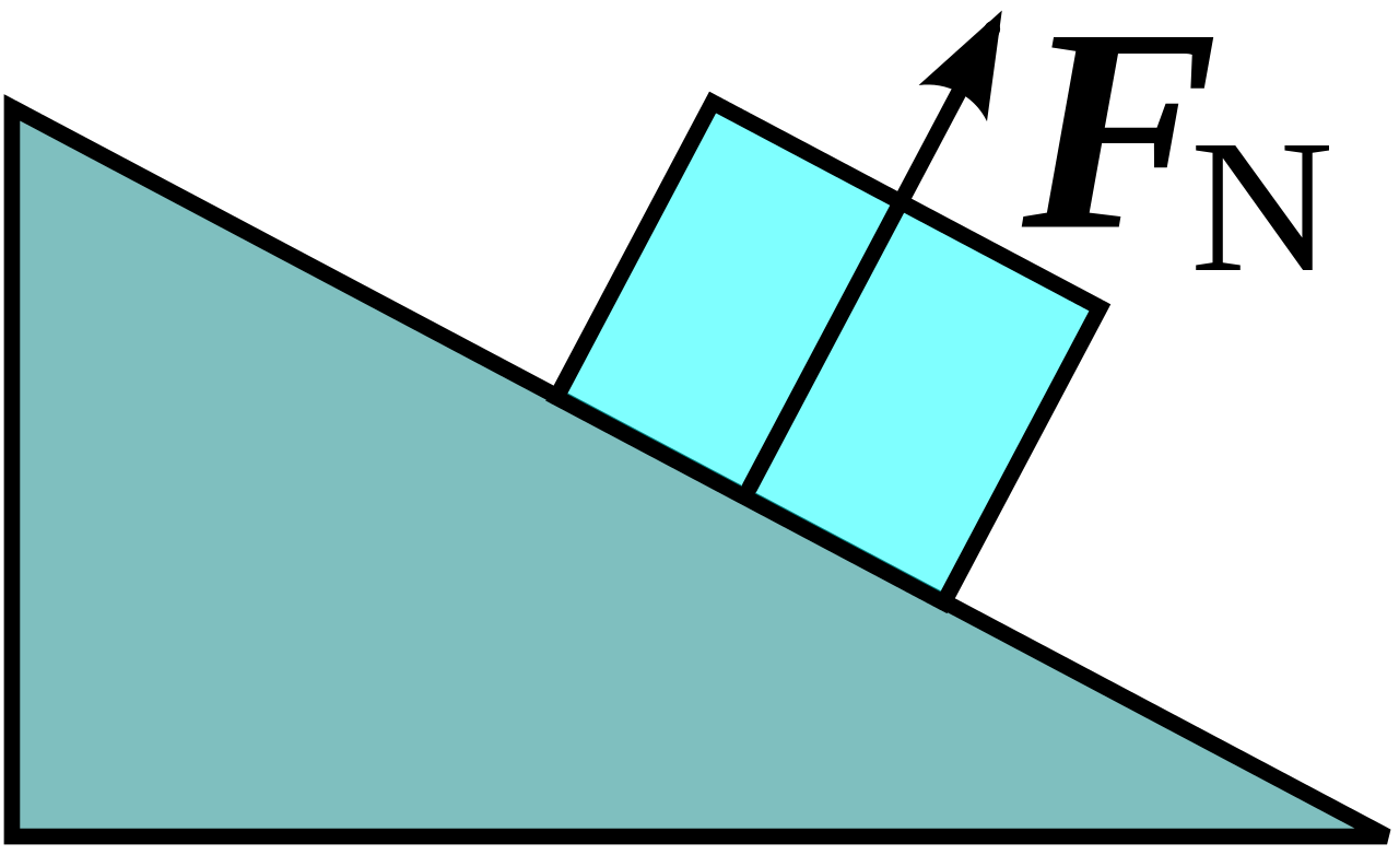
Normal force
The magnitude of the normal force $\b{F}_N$ is often denoted as $N$.
\[ \b{F}_N = N \hat{\b{n}} \]
where $\hat{\b{n}}$ is the unit vector normal to the surface.
Tension Force
The tension force is the force transmitted through a string, rope, or cable when it is pulled tight by forces acting from opposite ends. Tension is always directed along the length of the string or rope and pulls equally on both ends. The magnitude of the tension force $\b{F}_T$ is often denoted as $T$.
\[ \b{F}_T = T \hat{\b{l}} \]
where $\hat{\b{l}}$ is the unit vector in the direction of the string or rope.
Elastic Force
The elastic force is the restoring force exerted by a material when it is deformed (stretched or compressed) and tries to return to its original shape. The elastic force $\b{F}_e$ of an 1-dimensional elastic material is given by Hooke’s Law:
\[ \b{F}_e = -k \b{x} \]
where $k$ is the spring constant (a measure of the stiffness of the material) and $\b{x}$ is the displacement vector from the equilibrium position. The negative sign indicates that the force acts in the opposite direction of the displacement.
Frictional Force
The frictional force or dry friction is the force that opposes the relative motion of two surfaces in contact. The magnitude of the frictional force $\b{F}_f$ is often denoted as $f$.
\[ \b{F}_f = -f\hat{\b{v}} \]
where $\hat{\b{v}}$ is the unit vector in the direction of the relative motion between the surfaces. In microsopic terms, it is caused by the interactions between the microscopic irregularities of the surfaces in contact. Let’s take a look for the three laws of dry friction:
- Amontons’ First Law: The force of friction is directly proportional to the applied load.
- Amontons’ Second Law: The force of friction is independent of the apparent area of contact.
- Coulomb’s Law of Friction: Kinetic friction is independent of the sliding velocity.
By the laws of dry friction, we can model the frictional force as:
\[ f = \mu N \]
where $\mu$ is the coefficient of friction and $N$ is the normal force between the surfaces. We can observe that the coefficient of friction is a dimensionless scalar quantity. See the graph below for the relationship between the frictional force and the external horizontal force applied to the object.

Relationship between frictional force and external horizontal force
This is proven by numerous experiments, and it is a good approximation for many materials. Here, the normal force $N$ is assumed to be constant. By the graph, we can see that the frictional force is equal to the external horizontal force applied to the object until it reaches certain threshold. Until that threshold, the object is at rest since the net force acting on it is zero, so we call the friction at this state static friction. Upon reaching the threshold, the object starts to move, and the frictional force decreases to a constant value, which is called kinetic friction.
\[ f_s = \mu_s N \nl f_k = \mu_k N \]
where $f_s$ is the static frictional force, $f_k$ is the kinetic frictional force, $\mu_s$ is the coefficient of static friction, and $\mu_k$ is the coefficient of kinetic friction. The coefficient of static friction represents the maximum static frictional force before the object starts to move, and is usually greater than the coefficient of kinetic friction.
Block on a Ramp
When a block is placed on a ramp, the frictional force can be analyzed in terms of the angle of the ramp and the normal force. Let’s see the free body diagram of a block on a ramp:

Free body diagram of a block on a ramp
Let’s set the x-axis along the ramp and the y-axis perpendicular to the ramp. The forces acting on the block are the gravitational force, the normal force, and the frictional force. The gravitational force can be decomposed into two components: one parallel to the ramp and one perpendicular to the ramp. By the y-axis, the body will not move, so the net force in the y-direction is zero.
\[ \sum F_y = N - mg \cos \theta = 0 \implies N = mg \cos \theta \]
The frictional force acts in the opposite direction of the component of the gravitational force parallel to the ramp.
\[ \sum F_x = mg \sin \theta - f \]
Let’s seek for the condition for the block to be at rest.
\[ 0 = mg \sin \theta - f \geq mg \sin \theta - \mu_s N \nl \mu_s mg \cos \theta \geq mg \sin \theta \nl \therefore \; \theta \leq \tan^{-1} \mu_s \]
If the angle of the ramp $\theta$ is less than $\tan^{-1} \mu_s$, the block will not slide down the ramp. If not, the block will slide down the ramp, and the kinetic frictional force will act on the block.
\[ ma_x = mg \sin \theta - \mu_k N = mg \sin \theta - \mu_k mg \cos \theta \nl \therefore \; a_x = g (\sin \theta - \mu_k \cos \theta) \]
The block will slide down the ramp with an constant acceleration $a_x$.
Drag Force
The drag force is the resistance force experienced by an object moving through a fluid (liquid or gas). It acts in the opposite direction of the object’s velocity, and it makes the object reach a terminal velocity when the drag force equals the external force acting on the object. There are two main types of drag forces: Stokes drag and Newton drag.
Stokes Drag
Stokes drag is the drag force experienced by an object moving slowly through a viscous fluid. The Stokes drag force $\b{F}_d$ is given by:
\[ \b{F}_d = -k \b{v} \]
where $k$ is the Stokes drag coefficient, and $\b{v}$ is the velocity vector of the object. Let’s solve the equation of motion for an object experiencing Stokes drag and gravity.
\[ m \odv{}{t} \begin{bmatrix} v_x \nl v_y \end{bmatrix} = \begin{bmatrix} -k v_x \nl -mg -k v_y \end{bmatrix} \]
By substituting $\mu = k/m$, we can write the solution as:
\[ \begin{bmatrix} v_x \nl v_y \end{bmatrix} = \begin{bmatrix} v_{x0} e^{-\mu t} \nt -\dfrac{g}{\mu} + \left(v_{y0} + \dfrac{g}{\mu}\right) e^{-\mu t} \end{bmatrix} \]
\[ \begin{bmatrix} x \nl y \end{bmatrix} = \begin{bmatrix} \dfrac{v_{x0}}{\mu} \left(1 - e^{-\mu t}\right) \nt -\dfrac{g}{\mu}t + \dfrac{1}{\mu} \left(v_{y0} + \dfrac{g}{\mu}\right) \left(1 - e^{-\mu t}\right) \end{bmatrix} \]
where $v_{x0}$ and $v_{y0}$ are the initial velocities in the x and y directions, respectively. The terminal velocity is:
\[ \b{v}_t = -\frac{g}{\mu} \hat{\b{y}} \]
Newton Drag
Newton drag is the drag force experienced by an object moving at high speeds through a fluid. The Newton drag force $\b{F}_d$ is given by:
\[ \b{F}_d = -kv \b{v} = -k \b{v}^2 \hat{\b{v}} \]
where $k$ is the drag coefficient. Unlike Stokes drag, the drag force is proportional to the square of the velocity. Let’s solve the equation of motion for an object experiencing Newton drag and gravity.
\[ m \odv{}{t} \begin{bmatrix} v_x \nl v_y \end{bmatrix} = \begin{bmatrix} -k v_x \sqrt{v_x^2 + v_y^2} \nl -mg -k v_y \sqrt{v_x^2 + v_y^2} \end{bmatrix} \]
However, this equation is nonlinear and cannot be solved analytically. Instead, let’s solve for some special cases. We’ll use $\mu = k/m$ for simplicity.
1. Nearly horizontal motion
Here we suppose that $v_x > 0$. When the object is moving nearly horizontally, i.e. $\abs{v_x} \gg \abs{v_y}$, we can write the equation approximately as:
\[ \begin{align*} \odv{v_x}{t} &= -\mu v_x^2 \nl \odv{v_y}{t} &= -g - \mu v_x v_y \end{align*} \]
The solution is:
\[ v_x = \frac{1}{1/v_{x0} + \mu t} \nt x = \frac{1}{\mu} \ln(1 + \mu v_{x0} t) \]
However, this solution is only valid while $v_y$ is negligible compared to $v_x$, implying that for large $t$, the error in the solution will grow. Let’s keep solving the equation for $v_y$.
\[ \odv{v_y}{t} = -g - v_y \frac{\mu v_{x0}}{1 + \mu v_{x0} t} \]
The solution is:
\[ v_y = \left(v_{y0} + \frac{g}{2\mu v_{x0}} \right) \frac{1}{1 + \mu v_{x0} t} - \frac{g}{2\mu v_{x0}} (1+ \mu v_{x0} t) \nt y = \frac{1}{\mu v_{x0}} \left( v_{y0} + \frac{g}{2\mu v_{x0}} \right) \ln(1 + \mu v_{x0} t) - \frac{g}{4\mu^2 v_{x0}} \left[ (1 + \mu v_{x0} t)^2 -1 \right] \]
2. Vertical motion upwards
We can write the equation as:
\[ \odv{v_y}{t} = -g - \mu v_y^2 \]
The solution is:
\[ v_y = -\sqrt{\frac{g}{\mu}} \tan \left[ \sqrt{\mu g} t - \tan^{-1} \left( \sqrt{\frac{\mu}{g}} v_{y0} \right) \right] \nt y = \frac{1}{2\mu} \ln \left( 1 + \frac{\mu}{g} v_{y0}^2 \right) + \frac{1}{\mu} \ln \cos \left[ \sqrt{\mu g} t - \tan^{-1} \left( \sqrt{\frac{\mu}{g}} v_{y0} \right) \right] \]
This solution is valid until the object reaches its maximum height, $t = \dfrac{1}{\sqrt{\mu g}} \tan^{-1} \sqrt{\dfrac{\mu}{g}} v_{y0}$. When $v_x$ is not zero but still $\abs{v_y} \gg \abs{v_x}$, we can write the equation approximately as:
\[ \begin{align*} \odv{v_x}{t} &= -\mu v_x v_y \nl \odv{v_y}{t} &= -g - \mu v_y^2 \end{align*} \]
Here, the equation for $v_y$ is still the same as above, so the equation for $v_x$ is:
\[ v_x = v_{x0} \, e^{-\mu y} \]
The solution is:
\[ v_x = \frac{v_{x0}}{\sqrt{1 + \dfrac{\mu}{g} v_{y0}^2}} \sec \left[\sqrt{\mu g} t - \tan^{-1} \left( \sqrt{\frac{\mu}{g}} v_{y0} \right) \right] \nt x = \frac{v_{x0}}{\sqrt{ \mu g + \mu^2 v_{y0}^2 }} \ln \left\vert \frac{ \sec \left[\sqrt{\mu g} t - \tan^{-1} \left( \sqrt{\dfrac{\mu}{g}} v_{y0} \right) \right] + \tan \left[\sqrt{\mu g} t - \tan^{-1} \left( \sqrt{\dfrac{\mu}{g}} v_{y0} \right) \right] }{ \sqrt{\dfrac{\mu}{g}v_{y0}^2+1} - \sqrt{\dfrac{\mu}{g}} v_{y0} } \right\vert \]
This solution is valid when $t \ll \dfrac{1}{\sqrt{\mu g}} \tan^{-1} \sqrt{\dfrac{\mu}{g}} v_{y0}$.
3. Vertical motion downwards
We can write the equation as:
\[ \odv{v_y}{t} = -g + \mu v_y^2 \]
In this case, the object will eventually reach a terminal velocity, which is given by:
\[ \b{v}_t = -\sqrt{\frac{g}{\mu}} \hat{\b{y}} \]
The solution is:
- $\abs{v_{y0}} < \abs{\b{v}_t}$
\[ v_y = -\sqrt{\frac{g}{\mu}} \tanh \left[ \sqrt{\mu g} t - \tanh^{-1} \left( \sqrt{\frac{\mu}{g}} v_{y0} \right) \right] \nt y = \frac{1}{2\mu} \ln \left( 1 - \frac{\mu}{g} v_{y0}^2 \right) - \frac{1}{\mu} \ln \cosh \left[ \sqrt{\mu g} t - \tanh^{-1} \left( \sqrt{\frac{\mu}{g}} v_{y0} \right) \right] \]
- $\abs{v_{y0}} = \abs{\b{v}_t}$
\[ v_y = -\sqrt{\frac{g}{\mu}} \nt y = -\sqrt{\frac{g}{\mu}} t \]
- $\abs{v_{y0}} > \abs{\b{v}_t}$
\[ v_y = -\sqrt{\frac{g}{\mu}} \coth \left[ \sqrt{\mu g} t - \coth^{-1} \left( \sqrt{\frac{\mu}{g}} v_{y0} \right) \right] \nt y = \frac{1}{2\mu} \ln \left( \frac{\mu}{g} v_{y0}^2 - 1 \right) - \frac{1}{\mu} \ln \sinh \left[ \sqrt{\mu g} t - \coth^{-1} \left( \sqrt{\frac{\mu}{g}} v_{y0} \right) \right] \]
When $v_x$ is not zero but still $\abs{v_y} \gg \abs{v_x}$, we can do the same thing as in the previous case.
\[ v_x = v_{x0} \, e^{\mu y} \]
The solution is:
- $\abs{v_{y0}} < \abs{\b{v}_t}$
\[ v_x = \frac{v_{x0}}{\sqrt{1 - \dfrac{\mu}{g} v_{y0}^2}} \sech \left[\sqrt{\mu g} t - \tanh^{-1} \left( \sqrt{\frac{\mu}{g}} v_{y0} \right) \right] \nt x = \frac{v_{x0}}{\sqrt{ \mu g - \mu^2 v_{y0}^2 }}\Bigg[ \sin^{-1}\left(\sqrt{\frac{\mu}{g}}v_{y0}\right) + \sin^{-1} \tanh \left[\sqrt{\mu g} t - \tanh^{-1} \left( \sqrt{\frac{\mu}{g}} v_{y0} \right) \right] \Bigg] \]
- $\abs{v_{y0}} = \abs{\b{v}_t}$
\[ v_x = v_{x0} \, e^{-\sqrt{\mu g} t} \nt x = \frac{v_{x0}}{\sqrt{\mu g}} \left( 1 - e^{-\sqrt{\mu g} t} \right) \]
- $\abs{v_{y0}} > \abs{\b{v}_t}$
\[ v_x = \frac{v_{x0}}{\sqrt{\dfrac{\mu}{g} v_{y0}^2-1}} \csch \left[\sqrt{\mu g} t - \coth^{-1} \left( \sqrt{\frac{\mu}{g}} v_{y0} \right) \right] \nt x = \frac{v_{x0}}{\sqrt{ \mu^2 v_{y0}^2 - \mu g }} \ln \left\vert \frac{\coth\left[\sqrt{\mu g} t - \coth^{-1} \left( \sqrt{\dfrac{\mu}{g}} v_{y0} \right) \right] - \csch \left[\sqrt{\mu g} t - \coth^{-1} \left( \sqrt{\dfrac{\mu}{g}} v_{y0} \right) \right]}{ \sqrt{\dfrac{\mu}{g}}v_{y0} + \sqrt{\dfrac{\mu}{g} v_{y0}^2-1} } \right\vert \]
